1
Raymond K. Wong Franky Lam William M.
Shui
National ICT Australia,
{raymond.wong, franky.lam,
bill.shui}@nicta.com.au
H.3.2Information SystemsInformation Storage H.2.4.nTextual DatabasesXML Databases Algorithms, Design, Performance
When looking for a compact storage scheme for XML, there are several issues that need to be addressed. For example, it has to support fast operations, especially we are considering software applications that target people on the move. Moreover, if intensive compression methods are employed, they need to be optional and can be switched on or off due to low computation power of some mobile devices. In summary, from our experience, the major issues include:
In this paper, we propose a compact XML storage engine, called
ISX (for Integrated Succinct XML system), to store XML in a more
concise structure and address all of the above issues.
Theoretically, ISX uses an amount of space near the information
theoretic minimum on random trees. For a constant ![]() , where
, where
![]() , and a document with
, and a document with
![]() nodes, we need
nodes, we need
![]() bits to represent the topology
of the XML document. Node insertions can be handled in constant
time on average but worst case
bits to represent the topology
of the XML document. Node insertions can be handled in constant
time on average but worst case
![]() time, and all node navigation
operations take worst case
time, and all node navigation
operations take worst case
![]() time but constant time
on average.
time but constant time
on average.
The rest of this paper is organized as follows: Section 2 summarizes relevant work in the field. Section 3 presents the basics of ISX and its topology layer. The fast node navigation operators, the querying interfaces and the update mechanism are then described in detail in Section 4. Finally, Section 5 presents the experiment results and Section 6 concludes the paper.
Related work that share the same motivations with this paper includes Maneth et al [17], Tolani and Haritsa [22], Min et al [19] and Buneman et al [4]. Compared to XMill, XGrind [22] has a lower compression ratio but supports certain types of queries. XPRESS [19] uses reverse arithmetic encoding to encode tags using start/end regions. Both XGrind and XPRESS require top-down query evaluation, and do not support set-based query evaluation such as structural joins.
Buneman et al [4] separate the tree structure and its data. They then use bi-simulation to compress the documents that share the same sub-tree, however, they can only support node navigations in linear time. With a similar idea but different technique, Maneth et al [17,5] also compress XML by calculating the minimal sharing graph equivalent to the minimal regular tree grammar. In order to provide tree navigations, a DOM proxy that maintains runtime traversal information is needed [5]. Since only the compression efficiency was reported in the paper, both query and navigation performance of their proposed scheme are unclear.
Most XML storage schemes, such as [15,9,10,12], make use of interval and
preorder/postorder labeling schemes to support constant time
order lookup, but fail to address the issue of maintenance of
these labels during updates. Recently, Silberstein et al
[21]
proposed a data structure to handle ordered XML which guarantees
both update and lookup costs. Similarly, the L-Tree labeling
scheme proposed by Chen et al [6] addressed
the same problem and has the same time and space complexity as
[21],
however, they do not support persistent identifiers. The major
difference between our proposal and these two work is that we try
to minimize space usage while allowing efficient access, query
and update of the database. In this paper, we show that our
proposed topology representation costs linear space while
[21] costs
![]() space.
space.
The work most related to this paper regarding databases with efficient storage is from Zhang et al [23]. The succinct approach proposed by Zhang et al [23] targeted secondary storage, and used a balanced parentheses encoding for each block of data. Unfortunately, their summary and partition schemes support rank and select operations in linear time only. Their approach also uses the Dewey encoding for node identifiers in their indexes. The drawbacks of the Dewey encoding are significant: updates to the labels require linear time, and the size of the labels is also linear to the size of the database in the worst case. Thus, the storage of the topology can require quadratic space in the worst case.
Finally, there are several related proposals published recently, e.g. [9,8]. [9] show that all XPath axes can be handled using a preorder/postorder labeling. Instead of maintaining these two labels (i.e., two integers), our proposed scheme requires less than 3 bits per node to process all XPath axes, which is an attractive alternative for applications that are both space and performance conscious.
Ferragina et. al.[8] first shred the XML tree into a table of two columns, then sort and compress the columns individually. It does not offer immediate capability of navigating or searching XML data unless an extra index is built. However, the extra index will degrade the overall storage size (i.e., the compression ratio). Furthermore, the times for disk access and decompression of local regional blocks have been omitted from their experiments. As a result, the performance of actual applications may be different from what the experiments shown. Same as most other related work, data updates have been disregarded.
This section describes the storage layer of the ISX system. It consists of three layers, namely, topology layer, internal node layer, and leaf node layer. In Figure 3, the topology layer stores the tree structure of the XML document, and facilitates fast navigational accesses, structural joins and updates. The internal node layer stores the XML elements, attributes, and signatures of the text data for fast text queries. Finally the leaf node layer stores the actual text data. Text data can be compressed by various common compression techniques and referenced by the topology layer.
Jacobson [11] showed that the
lower bound space requirement for representing a binary tree is
![]() bits, where the Catalan number
bits, where the Catalan number ![]() is the number
of possible binary trees over
is the number
of possible binary trees over ![]() nodes.
nodes.
Our storage scheme is based on the balanced parentheses encoding from [14], representing the topology of XML. Different from [14], our topology layer (Figure 3) actually supports efficient node navigation and updates.
The balanced parentheses encoding used in tier 0 reflects the nesting of element nodes within any XML document and can be obtained by a preorder traversal of the tree: we output an open parenthesis when we encounter an opening tag and a close parenthesis when we encounter a closing tag. In Figure 3, the topology of a DBLP XML fragment shown in Figure 1 is represented in tier 0 using the balanced parentheses encoding. In our implementation, we use a single bit 0 to represent an open parenthesis and a single bit 1 to represent a close parenthesis.
We avoid any pointer based approach to link a parenthesis to
its label, as it would increase the space usage from ![]() to a less
desirable
to a less
desirable
![]() . As our representation of the
topology also does not include a
. As our representation of the
topology also does not include a ![]() bit
persistent object identifier for each node in the document, we
must find a way to link the open parenthesis of
bit
persistent object identifier for each node in the document, we
must find a way to link the open parenthesis of ![]() in tier 0 to the
actual label itself. To address this, we adopt from Munro's work
[20]
although they do not use balanced parentheses encoding. Instead,
they control the topology size by using multiple layers of
variable-sized pointers, and may require many levels of
indirection. In addition, we make the element structure an exact
mirror of the topology structure instead of mirroring to the
pointers. This allows us to find the appropriate label for a node
by simply finding the entry in the corresponding position at the
element structure. As mentioned earlier, a pointer based approach
would require space usage of
in tier 0 to the
actual label itself. To address this, we adopt from Munro's work
[20]
although they do not use balanced parentheses encoding. Instead,
they control the topology size by using multiple layers of
variable-sized pointers, and may require many levels of
indirection. In addition, we make the element structure an exact
mirror of the topology structure instead of mirroring to the
pointers. This allows us to find the appropriate label for a node
by simply finding the entry in the corresponding position at the
element structure. As mentioned earlier, a pointer based approach
would require space usage of
![]() , which is undesirable. The next
issue is to handle the variable length of XML element labels. We
adopt the approach taken in previous work [22,23], and maintain a
symbol table, using a hash table to map the labels into a domain
of fixed size. In the worst case, this does not reduce the space
usage, as every node can have its own unique label. In practice,
however, XML documents tend to have a very small number of unique
labels. Therefore, we can assume that the number of unique labels
used in the internal nodes (
, which is undesirable. The next
issue is to handle the variable length of XML element labels. We
adopt the approach taken in previous work [22,23], and maintain a
symbol table, using a hash table to map the labels into a domain
of fixed size. In the worst case, this does not reduce the space
usage, as every node can have its own unique label. In practice,
however, XML documents tend to have a very small number of unique
labels. Therefore, we can assume that the number of unique labels
used in the internal nodes (![]() ) is very small,
and essentially constant. This approach allows us to have fixed
size records in the internal node layer.
) is very small,
and essentially constant. This approach allows us to have fixed
size records in the internal node layer.
Note that each element in the XML document actually has two
available entries in the array, corresponding to the opening and
closing tags. We could thus make the size of each entry
![]() bits, and split the identifier
for each elements over its two entries. However, the two entries
are not in general adjacent to each other, and hence splitting
the identifier could slow down lookups as we would need to find
the closing tag corresponding to the opening tag and decrease
cache locality. Hence, we prefer to use entries of
bits, and split the identifier
for each elements over its two entries. However, the two entries
are not in general adjacent to each other, and hence splitting
the identifier could slow down lookups as we would need to find
the closing tag corresponding to the opening tag and decrease
cache locality. Hence, we prefer to use entries of ![]() bits and
leave the second entry set to zero; this also provides us with
some slack in the event that new element labels are used in
updates.
bits and
leave the second entry set to zero; this also provides us with
some slack in the event that new element labels are used in
updates.
Since text nodes are also leaf nodes, they are represented as
pairs of adjacent unused spaces in the internal node layer. We
thus choose to make use of this ``wasted'' space by storing a
hash value of the text node of size ![]() bits. This
can be used in queries which make use of equality of text nodes
such as /
bits. This
can be used in queries which make use of equality of text nodes
such as /![]() /*[year="2003"], by scanning the hash value
before scanning the actual data to significantly reduce the
lookup time. Since texts are treated independently from the
topology and node layers, they can be optionally compressed by
any compression schemes. Instead of employing more sophisticated
compression techniques such as BWT [8] that are relatively slow on
mobile devices, a standard LZW compression method (e.g., gzip) is
used in this paper.
/*[year="2003"], by scanning the hash value
before scanning the actual data to significantly reduce the
lookup time. Since texts are treated independently from the
topology and node layers, they can be optionally compressed by
any compression schemes. Instead of employing more sophisticated
compression techniques such as BWT [8] that are relatively slow on
mobile devices, a standard LZW compression method (e.g., gzip) is
used in this paper.
Given an arbitrary node ![]() of a large XML
document, a navigation operator should be able to traverse back
and forth the entire document via various step axes of node
of a large XML
document, a navigation operator should be able to traverse back
and forth the entire document via various step axes of node
![]() .
Some frequently used step axes for an XML document tree are
parent, first-child, next-sibling, previous-sibling, next-following and next-preceding. These step axes can then be used
to provide programming interfaces, such as the DOM API, for
external access to the XML database.
.
Some frequently used step axes for an XML document tree are
parent, first-child, next-sibling, previous-sibling, next-following and next-preceding. These step axes can then be used
to provide programming interfaces, such as the DOM API, for
external access to the XML database.
Node navigation operators are described by the pseudo-code in Algorithm 1, which shows a tight coupling between the ISX topology layer primitives and the navigation operators. Each navigation operator in Algorithm 1 is mapped to a sequence of calls to the topology layer primitives described in Algorithm 2.
Node navigation operators are highly dependent on topology layer primitives such as FORWARDEXCESS and BACKWARDEXCESS. In the worst case, node navigation operators could take linear time. However, we can significantly improve the performance of the topology layer primitives by adding auxiliary data structures (tier 1 and tier 2 blocks) on top of the tier 0 layer described in Section 3.1.
Figure 4 presents the auxiliary tiers
1 (![]() ) and 2 (
) and 2 (![]() ), where each tier contains contiguous arrays
of tuples, with each tuple holding summary information of one
block in the lower tier. The tier 0 in the figure corresponds to
the balanced parentheses encoding of
the topology of the XML document, which was described in Section
3. For tiers 1 and 2, each tier 1
block stores an array of tier 0 tuples
), where each tier contains contiguous arrays
of tuples, with each tuple holding summary information of one
block in the lower tier. The tier 0 in the figure corresponds to
the balanced parentheses encoding of
the topology of the XML document, which was described in Section
3. For tiers 1 and 2, each tier 1
block stores an array of tier 0 tuples
![]() , where
, where ![]() is the maximum
number of tuples allowed per tier 1 block. Each
is the maximum
number of tuples allowed per tier 1 block. Each ![]() for
for
![]() is defined as
is defined as
![]() and the
density of each tier 0 block can be calculated by using the
formula
and the
density of each tier 0 block can be calculated by using the
formula
![]() . For
each tier 0 tuple,
. For
each tier 0 tuple, ![]() is the total number of left parentheses of a
block;
is the total number of left parentheses of a
block; ![]() is the total number of right parentheses of a
block;
is the total number of right parentheses of a
block; ![]() is the minimum excess within a single block by
traversing the parentheses array forward from the beginning of
the block;
is the minimum excess within a single block by
traversing the parentheses array forward from the beginning of
the block; ![]() is the maximum excess within a single block by
traversing the parentheses array forward from the beginning of
the block;
is the maximum excess within a single block by
traversing the parentheses array forward from the beginning of
the block; ![]() is the minimum excess within a single block by
traversing the parentheses array backward from the last
parenthesis of the block;
is the minimum excess within a single block by
traversing the parentheses array backward from the last
parenthesis of the block; ![]() is the maximum
excess within a single block by traversing the parentheses array
backward from the last parenthesis of the block; and
is the maximum
excess within a single block by traversing the parentheses array
backward from the last parenthesis of the block; and ![]() is total
number of character data nodes. In tier 2, each block stores an
array of tier 1 tuples
is total
number of character data nodes. In tier 2, each block stores an
array of tier 1 tuples
![]() , where
, where ![]() is the maximum
number of tuples allowed per tier 2 block, Each tuple
is the maximum
number of tuples allowed per tier 2 block, Each tuple
![]() for
for
![]() is then defined as
is then defined as
![]() , where:
, where:
![]() is the sum of all
is the sum of all ![]() for all tier 1 tuples
for all tier 1 tuples ![]() (
(
![]() );
);
![]() is the sum of all
is the sum of all ![]() for all tier 1 tuples
for all tier 1 tuples ![]() (
(
![]() );
);
![]() is the local forward minimum excess across all of its tier 1
tuples;
is the local forward minimum excess across all of its tier 1
tuples; ![]() is the local forward maximum excess across all
of its tier 1 tuples;
is the local forward maximum excess across all
of its tier 1 tuples; ![]() is the local backward minimum excess
across all of its tier 1 tuples;
is the local backward minimum excess
across all of its tier 1 tuples; ![]() is the local
backward maximum excess across all of its tier 1 tuples; and
is the local
backward maximum excess across all of its tier 1 tuples; and
![]() is the total number of character data nodes for all tier 1 tuples
(
is the total number of character data nodes for all tier 1 tuples
(
![]() ).
).
Although both tier 1 and tier 2 tuples look similar, the
values of ![]() ,
, ![]() ,
, ![]() and
and
![]() in tier 2 are calculated differently to that of in tier 1. For
tier 2, the function TIER2LOCALEXCESS
in Algorithm 3 is used to calculate the
local minimum/maximum excess and it is not as trivial as the
calculation for tier 1 blocks.
in tier 2 are calculated differently to that of in tier 1. For
tier 2, the function TIER2LOCALEXCESS
in Algorithm 3 is used to calculate the
local minimum/maximum excess and it is not as trivial as the
calculation for tier 1 blocks.
Let
![]() be a tier 2 tuple holding the
summary information for the tier 1 tuples
be a tier 2 tuple holding the
summary information for the tier 1 tuples
![]() . To calculate the local forward
minimum excess
. To calculate the local forward
minimum excess ![]() , we know the local minimum excess from the
beginning of the first parentheses of
, we know the local minimum excess from the
beginning of the first parentheses of ![]() until the end
of
until the end
of ![]() is equal to
is equal to ![]() , we then assign this value to
, we then assign this value to ![]() . We know the
excess at the end of
. We know the
excess at the end of ![]() is
is ![]() , so the
minimum of
, so the
minimum of ![]() and
and
![]() gives the forward minimum excess
from beginning parenthesis of
gives the forward minimum excess
from beginning parenthesis of ![]() to the end
parenthesis of
to the end
parenthesis of ![]() . Similarly, the minimum of
. Similarly, the minimum of
![]() gives the minimum excess between the beginning parenthesis of
gives the minimum excess between the beginning parenthesis of
![]() to the end parenthesis of
to the end parenthesis of ![]() . Therefore,
. Therefore,
![]() can be calculated by scanning its tier 1 tuples, updating the
excess along the way. Both maximum and minimum forward excesses
can be calculated at the same time. For backward excesses, the
algorithm is identical, except for the direction of traversal of
the tier 1 tuples.
can be calculated by scanning its tier 1 tuples, updating the
excess along the way. Both maximum and minimum forward excesses
can be calculated at the same time. For backward excesses, the
algorithm is identical, except for the direction of traversal of
the tier 1 tuples.
In the ISX system, the fixed block size for each tier is 4
kilobytes in size. Therefore, each tier 0 block can hold up to
32768 bits and each tier 1 block can hold
![]() tier 0 blocks.
Similarly, each tier 2 block can hold up to
tier 0 blocks.
Similarly, each tier 2 block can hold up to
![]() tier 1 blocks,
which is equivalent to
tier 1 blocks,
which is equivalent to
![]() tier 0
blocks. For a 32-bit word machine, there are only 2 tier 2 blocks
and in theory, there are
tier 0
blocks. For a 32-bit word machine, there are only 2 tier 2 blocks
and in theory, there are
![]() tier 2 blocks. Therefore, the
worst case for navigational accesses is
tier 2 blocks. Therefore, the
worst case for navigational accesses is
![]() , which is not much of an
improvement on
, which is not much of an
improvement on ![]() . Fortunately, it is relatively simple to fix
this limitation: instead of having
. Fortunately, it is relatively simple to fix
this limitation: instead of having ![]() tiers, we
generalize the above structure in a straightforward fashion to
use
tiers, we
generalize the above structure in a straightforward fashion to
use
![]() tiers. This means that the
top-most tier has
tiers. This means that the
top-most tier has
![]() blocks, reducing the worst case navigational access time to
blocks, reducing the worst case navigational access time to
![]() .
.
FORWARDEXCESS and
BACKWARDEXCESS
return the position of the first parenthesis matching the given
excess ![]() within a given range
within a given range
![]() (in forward and backward direction
respectively).
(in forward and backward direction
respectively).
Using the auxiliary structures (tiers 1 and 2), instead of
just a linear scan of tier 0 layer, we can use tier 1 to test
whether the position of the parenthesis, matching ![]() excess, lies
within the
excess, lies
within the ![]() -th tier 0 block, i.e., checking whether
-th tier 0 block, i.e., checking whether
![]() , where
, where
![]() is the excess between
is the excess between ![]() and the beginning of the
and the beginning of the ![]() -th tier 0 block
(excluding the first bit). However, as
-th tier 0 block
(excluding the first bit). However, as
![]() , there are potentially
, there are potentially
![]() tier 1 tuples to scan. Hence, we
use tier 2 find the appropriate tier 1 block within which
tier 1 tuples to scan. Hence, we
use tier 2 find the appropriate tier 1 block within which
![]() lies, thus reducing the cost to a near
constant in practice.
lies, thus reducing the cost to a near
constant in practice.
Using the above approach, we can replace primitives
NEXT, FORWARDEXCESS and
BACKWARDEXCESS in
Algorithm 2 with improved primitives in
Algorithm 4. Furthermore, since the
depths of real-world XML documents are generally less than
![]() (even the depth of the highly nested
Tree Bank dataset [18] is much less than 100),
most matching parentheses lie within the same block, and
occasionally are found in neighboring blocks. Therefore, when
FASTFORWARDEXCESS
is called from navigation operations, we rarely need to access
additional blocks in either the auxiliary data structure or the
topology bit array. In the worst case, when the matching
parentheses lie within different blocks, we only need to read two
tier 1 blocks and two tier 2 blocks for a 32-bit word size
machine, which is very small in size.
(even the depth of the highly nested
Tree Bank dataset [18] is much less than 100),
most matching parentheses lie within the same block, and
occasionally are found in neighboring blocks. Therefore, when
FASTFORWARDEXCESS
is called from navigation operations, we rarely need to access
additional blocks in either the auxiliary data structure or the
topology bit array. In the worst case, when the matching
parentheses lie within different blocks, we only need to read two
tier 1 blocks and two tier 2 blocks for a 32-bit word size
machine, which is very small in size.
In ISX system, we also facilitate efficient update operators, such as node insertion. So far for tier 0 layer, we have appeared to treat the balanced parentheses encoding as a contiguous array. This scheme is not suitable for frequent updates as any insertion or deletion of data would require shifting of the entire bit array.
In this section, we present the modification to our storage
scheme, that changes the space usage from ![]() to
to
![]() , where
, where
![]() , so that we can efficiently
accommodate frequent updates.
, so that we can efficiently
accommodate frequent updates.
![\includegraphics[width=0.8\textwidth]{f_order}](fp794-wong-html-img90.png)
|
In our approach, we first divide the array into blocks of
![]() bits each, and store the blocks
contiguously. Within each block, we leave some empty space by
storing them at the rightmost portion of each block. Now, we only
need to shift
bits each, and store the blocks
contiguously. Within each block, we leave some empty space by
storing them at the rightmost portion of each block. Now, we only
need to shift ![]() entries per insertion or deletion.
We can control the cost of shifting by adjusting the block
size.
entries per insertion or deletion.
We can control the cost of shifting by adjusting the block
size.
After the initial loading of an XML document, the empty space
allocated to leaf nodes will eventually be used up as more data
is inserted into the database. Therefore, we need to guarantee an
even distribution of empty bits across the entire parentheses
array, so that we can still maintain the ![]() bound for the number of shifts needed for each data insertion.
This can be achieved by deciding exactly when to redistribute
empty space among the blocks and which blocks are to be involved
in the redistribution process.
bound for the number of shifts needed for each data insertion.
This can be achieved by deciding exactly when to redistribute
empty space among the blocks and which blocks are to be involved
in the redistribution process.
To better understand our approach, we first visualize these
blocks as leaf nodes of a virtual balanced
binary trie, with the position of the block in the array
corresponding to the path to that block through the virtual
binary trie. Figure 5 shows such a trie,
where block 0 corresponds to the leaf node under the path
![]() , and similarly block 3
corresponds to the path
, and similarly block 3
corresponds to the path
![]() . For each block, we define:
. For each block, we define:
Given the above definition of density for leaf nodes, the
density of a virtual node is the average density of its
descendant leaf nodes. We then control the empty space within all
nodes in the virtual binary trie by setting a density threshold
![]() , within which the block densities must
lie. For a virtual node at height
, within which the block densities must
lie. For a virtual node at height ![]() and depth
and depth
![]() in the virtual trie, we enforce a density threshold of
in the virtual trie, we enforce a density threshold of
![]() . For example, the density threshold range for virtual node
. For example, the density threshold range for virtual node
![]() in Figure 5 is
in Figure 5 is
![]() , since the depth for
, since the depth for ![]() is 2 and height of the trie is 3.
is 2 and height of the trie is 3.
Why do we use the formula above for
controlling the density threshold? This is due to two
factors: first, in order to guarantee good space utilization, the
maximum density of a leaf node should be 1, and the minimum
density threshold of root node should be ![]() . Secondly,
the density threshold should satisfy the following invariant: the
density threshold range of an ancestor node should be tighter
than the range for its descendant nodes. This is so that space
redistribution for an ancestor node
. Secondly,
the density threshold should satisfy the following invariant: the
density threshold range of an ancestor node should be tighter
than the range for its descendant nodes. This is so that space
redistribution for an ancestor node ![]() , the density
threshold of all its descendants are also immediately
satisfied.
, the density
threshold of all its descendants are also immediately
satisfied.
In the worst case, we use ![]() bits per node,
since the root node can be only half full. Thus, on a
bits per node,
since the root node can be only half full. Thus, on a
![]() -bit word machine, we can store at most
-bit word machine, we can store at most
![]() nodes. However, by adjusting the
minimum root node density threshold, from
nodes. However, by adjusting the
minimum root node density threshold, from
![]() to
to
![]() it is possible to store more
than
it is possible to store more
than ![]() nodes by choosing a smaller
nodes by choosing a smaller ![]() . In
practice,
. In
practice, ![]() should be
should be ![]() and therefore
and therefore
![]() bits is in effect
bits is in effect ![]() . The factor
. The factor
![]() should only be less than
should only be less than ![]() when the
document is relatively static.
when the
document is relatively static.
Notice that although we shift the parentheses within tier 0
during update, we never need to shift the tuples in tier 1
because the same ![]() tuple always corresponds to the same tier 0
block, regardless of its density. Therefore unlike tier 0, we do
not need to redistribute tuples within tier 1 (similarly for tier
2) during the update operation.
tuple always corresponds to the same tier 0
block, regardless of its density. Therefore unlike tier 0, we do
not need to redistribute tuples within tier 1 (similarly for tier
2) during the update operation.
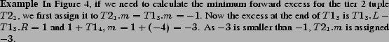
![\begin{algorithm} % latex2html id marker 357 [!!bp] \begin{center} \caption{ Off... ...1_x+4\lg\vert\B\vert)$ \end{tabbing}}} \end{center}\vspace{-3mm} \end{algorithm}](fp794-wong-html-img116.png)
From Section 4.2, the auxiliary
tiers may first appear to increase the update costs to
![]() , since moving a node
requires updating
, since moving a node
requires updating
![]() tiers. However, this overhead
can be eliminated by updating the upper tiers once per
redistribution, instead of once per node. A simple proof then
demonstrates that the overall update cost is unaffected, and
remains
tiers. However, this overhead
can be eliminated by updating the upper tiers once per
redistribution, instead of once per node. A simple proof then
demonstrates that the overall update cost is unaffected, and
remains
![]() .
.
During the insertions and deletions in a tier 0 block, we simply update the appropriate tuples in the corresponding blocks in the higher tiers. Since the redistribution process we described in Section 4.4.1 can be seen as a sequence of insertions and deletions, the corresponding updates to the auxiliary tiers do not affect the worst case complexity for updates.
Having
![]() bits used per node including update,
using 32-bits word, we can store as much as
bits used per node including update,
using 32-bits word, we can store as much as ![]() nodes. In
our implementation we also chose to use four kilobytes sized
block. Based on these values, we now discuss the space cost of
each component of our storage scheme. Of course, if larger
documents need to be stored, we can increase the word size that
we use in the data structure and adjust the bit length used on
tier 1 and tier 2.
nodes. In
our implementation we also chose to use four kilobytes sized
block. Based on these values, we now discuss the space cost of
each component of our storage scheme. Of course, if larger
documents need to be stored, we can increase the word size that
we use in the data structure and adjust the bit length used on
tier 1 and tier 2.
 tier 2 blocks to store the 449 tier 1 tuples.
Since we only need a maximum of two tier 2 blocks, even for
![]() nodes document, we can just keep them in
main memory. In fact, the entire tier 1 can also be kept in main
memory, since it requires at most
nodes document, we can just keep them in
main memory. In fact, the entire tier 1 can also be kept in main
memory, since it requires at most
![]() . In summary, the
space required by the topology layer (in bits) is:
. In summary, the
space required by the topology layer (in bits) is:
and the space required by the internal node layer (in bits)
plus the symbol table is:
![]()
We can use the above equations to estimate the space used by
an XML file, using as our example a 100 MB copy of DBLP, which
was roughly 5 million nodes. If we assume there are no updates
after the initial loading, we can set
![]() . According to the equation, we will
have used roughly
. According to the equation, we will
have used roughly
![]() for the topology
layer, and
for the topology
layer, and
![]() . This, of
course, disregards the space needed for the text data in the
document.
. This, of
course, disregards the space needed for the text data in the
document.
Based on the block size ![]() , we
know the exact size of tuples and tiers in our topology layer.
Therefore, given a bit position
, we
know the exact size of tuples and tiers in our topology layer.
Therefore, given a bit position ![]() , we
can calculate which tier 0 block this bit belongs to and which
tier 1 block contains summary information for the tier 0 block.
For a given
, we
can calculate which tier 0 block this bit belongs to and which
tier 1 block contains summary information for the tier 0 block.
For a given ![]() , Algorithm 6
lists all the calculations needed to find its resident tier 0 to
tier 2 blocks and the index within the blocks to get the
summary.
, Algorithm 6
lists all the calculations needed to find its resident tier 0 to
tier 2 blocks and the index within the blocks to get the
summary.
|
The ISX system is implemented in C++ using Expat XML parser1. In this section, we compare the performance of ISX with other related implementations, namely, XMill [16], XGrind [22], NoK [23] and TIMBER [12]. Experiments were setup to measure various performances according to the feature matrix of these implementations as shown in Table 1.
We used an Apple G5 2.0 GHz machine with 2.5GB RAM and 160GB
of 7,200 RPM IDE hard drive. The memory buffer pool of ISX has
been fixed to 64MB for all the experiments. Three XML datasets
were used, namely, DBLP [1], Protein Sequence Database
(PSD) [3], TreeBank
[18]. We found that
the experiment results from PSD are very similar to those from
DBLP due to their regular, shallow tree structure. Therefore, PSD
results are skipped from some plots below for clarity. Large
datasets (i.e., ![]() 1GB) were generated by repeatedly duplicating
and merging the source dataset, e.g., the 16GB DBLP document
contains more than 770 million nodes.
1GB) were generated by repeatedly duplicating
and merging the source dataset, e.g., the 16GB DBLP document
contains more than 770 million nodes.
|
Table 2 and 3 show that XMill has the best compression ratio for both DBLP and TreeBank datasets. Compared to XMill that does not support any direct data navigation and queries, XGrind does allow simple path expressions. Therefore, it has a relatively less attractive compression ratio. In fact, XGrind failed to run on large datasets in our experiments. Both XMill and XGrind have better space consumption as they are primarily designed for read-only data and do not support efficient updates. Furthermore, they only support access to the compressed data in linear time.
Table 2 and 3 show again that ISX is relatively less sensitive to the structure of the data. Although the compression ratio of ISX for TreeBank is not as good as for DBLP, the reason is that TreeBank has the text content that are harder to compress (TreeBank text are more random than the DBLP's). XMill compression ratio on TreeBank is relatively much worse than that on DBLP is due to both the random text content as well as the more complex tree structure of the data.
The performance comparison of bulk loading using ISX, NoK, XGrind and XMill are shown in Figure 6. For the smaller datasets (up to 500MB DBLP), Figure 6(a) shows our ISX system significantly outperforms NoK and TIMBER in loading. It also highlights the scalability of ISX in loading large datasets.
[ISX vs. TIMBER and NoK (up to 500
MB data)]![\includegraphics[width=0.8\textwidth]{isx_vs_timber_loading_time_line}](fp794-wong-html-img138.png) [ISX vs. XGrind and XMill (up to 16 GB data)] ![\includegraphics[width=0.8\textwidth]{load_time}](fp794-wong-html-img139.png)
|
To further test the scalability of loading even larger XML documents, we compared the loading time of ISX and the other well known systems such as XMill and XGrind on 1 to 16 GB of DBLP documents. During the loading process, XGrind failed to load XML documents greater than 100MB. Although Figure 6(b) shows that the loading time for ISX is slower than XMill's, it still exhibits a similar trend (similar scalability). The gap between the two curves is contributed by the fact that ISX does not compress the XML data as much as XMill does. This results in a larger storage layer than XMill, which will then uses higher number of disk writes.
When consider using the proposed structure as a storage scheme of a full-fledged database system, one must consider its query performance. Figure 7 (with details listed in Tables 4) shows the query performance of ISX against other schemes. Note that the query times in Figure 7 are in logarithmic scale. From this experiment, we found that ISX outperforms other systems in either the ISX or ISX Stream (using the TurboXPath approach [13]) modes. The performance of ISX is measured by using binary structural join to perform XPath queries; while ISX Stream execute the same query by scanning ISX topology layer linearly.
[DBLP Q1]![\includegraphics[width=0.8\textwidth]{isx_vs_timber_dblp1}](fp794-wong-html-img148.png) [DBLP Q2] ![\includegraphics[width=0.8\textwidth]{isx_vs_timber_dblp2}](fp794-wong-html-img149.png) [DBLP Q3] ![\includegraphics[width=0.8\textwidth]{isx_vs_timber_dblp3}](fp794-wong-html-img150.png) [DBLP Q4] ![\includegraphics[width=0.8\textwidth]{isx_vs_timber_dblp5}](fp794-wong-html-img151.png) [DBLP Q5] ![\includegraphics[width=0.8\textwidth]{isx_vs_timber_dblp6}](fp794-wong-html-img152.png) [DBLP Q6] ![\includegraphics[width=0.8\textwidth]{isx_vs_timber_dblp8}](fp794-wong-html-img153.png)
|
[Node navigation time
(microseconds)]![\includegraphics[width=0.8\textwidth]{nav}](fp794-wong-html-img154.png) [Full document traversal time (seconds)] ![\includegraphics[width=0.8\textwidth]{traverse}](fp794-wong-html-img155.png)
|
To test the performance and scalability of random node navigation, we pre-loaded our XML datasets, and for each database, we randomly picked a node and called the node traversal functions (e.g., FIRSTCHILD, NEXTSIBLING) multiple times. The average access time for these node traversal operations are plotted in Figure 8(a). The graph shows that as the database size gets bigger, the running time for these functions remains constant. This is not surprising, since in general most nodes are located close to their siblings, and hence are likely to be in the same block. For example, it generally only takes a scan of a few bits on average to access either the first child node or the next sibling node. Some operations are faster than the others, due to their different implementation complexity (listed in Algorithm 1) and the characteristics of the encoding itself. For instance, as Figure 8(a) shows, FIRSTCHILD performed slightly faster than NEXTSIBLING function, because the first child is always adjacent to a node, whereas its next sibling might be several nodes away.
With fast traversal operations, ISX can traversal XML data in the proposed compact encoding significantly faster than other XML compression techniques such as XMill, as shown in Figure 8(b). We argue that this feature is important to examine the content of large XML databases or archives.
The worst case for Algorithm 5
happens when nodes are inserted at the beginning of a completely
packed database, i.e., with no gaps between blocks. The insertion
experiment was set to measure its average worst case performance
by inserting nodes at the beginning of the database. For each
experiment, we did multiple runs (resetting the database after
each run). The average insertion times (per node) are shown in
Figures 9. In Figure 9, we see an initial spike in the execution
time for the worst case insertion. This corresponds to the
initial packed state of the database, in which case the very
first node insertion requires the redistribution of the entire
leaf node layer. Clearly, in practice this is extremely unlikely
to happen, but the remainder of the graph demonstrates that even
this contrived situation has little effect on the overall
performance. The graph also shows that the cost of all subsequent
insertions increases at a rate of approximately
![]() . In fact, all subsequent insertions
up to 100,000 took no more than 0.5 milliseconds.
. In fact, all subsequent insertions
up to 100,000 took no more than 0.5 milliseconds.
Updating the values of nodes will not cause extra processing time apart from the retrieval time for locating the nodes to be updated. In case of deletion, the reverse sequence of steps for node insertion will be performed (freed space will be left as gaps to be filled by subsequent insertions).
A compact and efficient XML repository is critical for a wide range of applications such as mobile XML repositories running on devices with severe resource constraints. For a heavily loaded system, a compact storage scheme could be used as an index storage that can be manipulated entirely in memory and hence substantially improve the overall performance. In this paper, we proposed a scalable and yet efficient, compact storage scheme for XML data.
Our data structure is shown to be exceptionally concise, without sacrificing query and update performance. While having the benefits of small data footprint, experiments have shown that the proposed structure still out-performs other XML database systems and scales significantly better for large datasets. In particular, all navigational primitives can run in near constant time. Furthermore, as shown in the experiments, our proposed structure allows direct document traversal and queries that are significantly faster and more scalable than previous compression techniques.
![\includegraphics[width=0.8\textwidth]{f_xml}](fp794-wong-html-img11.png)
![\includegraphics[width=0.8\textwidth]{f_overview}](fp794-wong-html-img12.png)
![\includegraphics[width=0.8\textwidth]{f_parentheses}](fp794-wong-html-img13.png)
![\begin{definition} % latex2html id marker 149 [Definition:] \par \emph{An excess... ...en parenthesis of $x$\ and the beginning of the document.} \par \end{definition}](fp794-wong-html-img16.png)
![\begin{algorithm} % latex2html id marker 161 [h!bp] \begin{center} \caption{ Nod... ... \ 3\>\RETURN $follow$ \end{tabbing}} \end{center}\vspace{-3mm} \end{algorithm}](fp794-wong-html-img26.png)
![\begin{algorithm} % latex2html id marker 184 [!!bp] \begin{center} \caption{ Pri... ...t tier0\vert$, $0$) \ \end{tabbing}} \end{center}\vspace{-3mm} \end{algorithm}](fp794-wong-html-img27.png)
![\includegraphics[width=0.8\textwidth]{f_tiers}](fp794-wong-html-img28.png)
![\begin{algorithm} % latex2html id marker 212 [!!bp] \begin{center} \caption{ Cal... ...1[t1].L - tier1[t1].R$ \end{tabbing}}} \end{center}\vspace{-3mm} \end{algorithm}](fp794-wong-html-img29.png)
![\begin{algorithm} % latex2html id marker 262 [h!bp] \begin{center} \caption{ Top... ...in backward direction. \end{tabbing}}} \end{center}\vspace{-3mm} \end{algorithm}](fp794-wong-html-img76.png)
![\begin{algorithm} % latex2html id marker 333 [tbp] \begin{center} \caption{ Node... ...er 1 and tier 2 tuples. \end{tabbing}} \end{center}\vspace{-3mm} \end{algorithm}](fp794-wong-html-img106.png)
![\includegraphics[width=0.8\textwidth]{updates}](fp794-wong-html-img156.png)